Code Walkthrough: A use case of YY1 and YY2 in HeLa cells
Mahmoud Ahmed1
2020-12-16
Source:vignettes/workshop_code.Rmd
workshop_code.Rmd
# load required libraries
library(dplyr)
library(tidyr)
library(readr)
library(purrr)
library(GenomicRanges)
library(rtracklayer)
library(AnnotationDbi)
library(TxDb.Hsapiens.UCSC.hg19.knownGene)
library(org.Hs.eg.db)
library(target)
Motivation
YY1 and YY2 belongs to the same family of transcription factors.
-
Ying Yang 1 (YY1)
- A zinc finger protein
- Direct deacetylase and histone acetyltransferases of many promoters
- Induces or represses the expression of the target genes
-
Ying Yang 2 (YY2)
- A zinc finger protein
- Arose by retro-transposition of YY1
Using the target analysis, we will attempt to answer the following questions:
- Do the two transcription factors share the same target genes?
- What are the consequences of the binding of each factor on its targets?
- On the shared targets, how the two factors functionally interact?
Datasets
To answer these questions, we use publicly available datasets.
Table 1. Expression and binding data of YY1 and YY2 in HeLa cells.
| GEO ID | Data Type | Design | Ref. |
|---|---|---|---|
| GSE14964 | Microarrays | YY#-knockdown | Chen et al. (2010) |
| GSE31417 | ChIP-Seq | YY1 vs input | Michaud et al. (2013) |
| GSE96878 | ChIP-Seq | YY2 vs input | Wu et al. (2017) |
Data pre-processing:
- Microarrays were obtained in the form of differential expression between the two conditions from KnockTF.
- The ChIP peaks were obtained in the form of
bedfiles from ChIP-Atlas. - USSC hg19 human genome to extract the genomic annotation
Data analysis:
- Prepare the three sources of data for the target analysis
- Predict the specific targets for each individual factors
- Predict the combined function of the two factors on the shared target genes
Preparing the binding data
The ChIP peaks were downloaded in the form of separate bed files for each factor. We first locate the files in the data/ directory and load the files using import.bed. Then the data is transformed into a suitable format, GRanges. The resulting object, peaks, is a list of two GRanges items, one for each factor.
# locate the peaks bed files
peak_files <- c(YY1 = 'data/Oth.Utr.05.YY1.AllCell.bed',
                YY2 = 'data/Oth.Utr.05.YY2.AllCell.bed')

# load the peaks bed files as GRanges
peaks <- map(peak_files, ~GRanges(import.bed(.x)))
# show the numbers of peaks of the two factors
lengths(peaks)
#>   YY1   YY2
#> 31490  3368

# show the first few entries of the GRanges object
show(peaks$YY1)
#> GRanges object with 31490 ranges and 4 metadata columns:
#>           seqnames            ranges strand |                   name     score
#>              <Rle>         <IRanges>  <Rle> |            <character> <numeric>
#>       [1]     chr1        9980-10149      * | ID=SRX092576;Name=YY..       186
#>       [2]     chr1       10001-10265      * | ID=SRX190209;Name=YY..       512
#>       [3]     chr1       10368-10452      * | ID=SRX190209;Name=YY..       128
#>       [4]     chr1       11219-11322      * | ID=SRX190209;Name=YY..       100
#>       [5]     chr1       29140-29432      * | ID=SRX190209;Name=YY..       418
#>       ...      ...               ...    ... .                    ...       ...
#>   [31486]     chrY 58996509-58996690      * | ID=SRX092576;Name=YY..       135
#>   [31487]     chrY 58996927-58997108      * | ID=SRX092576;Name=YY..       183
#>   [31488]     chrY 58996934-58997092      * | ID=SRX190209;Name=YY..       111
#>   [31489]     chrY 59363025-59363426      * | ID=SRX190209;Name=YY..       894
#>   [31490]     chrY 59363027-59363397      * | ID=SRX092576;Name=YY..       404
#>               itemRgb             thick
#>           <character>         <IRanges>
#>       [1]     #00BDFF        9980-10149
#>       [2]     #0CFF00       10001-10265
#>       [3]     #0082FF       10368-10452
#>       [4]     #0066FF       11219-11322
#>       [5]     #00FF53       29140-29432
#>       ...         ...               ...
#>   [31486]     #0089FF 58996509-58996690
#>   [31487]     #00BAFF 58996927-58997108
#>   [31488]     #0071FF 58996934-58997092
#>   [31489]     #FF6C00 59363025-59363426
#>   [31490]     #00FF61 59363027-59363397
#>   -------
#>   seqinfo: 56 sequences from an unspecified genome; no seqlengths

# show number of peaks in each chromosome
table(seqnames(peaks$YY1))
#>
#>                  chr1                 chr10                 chr11
#>                  3126                  1632                  1590
#>                 chr12                 chr13                 chr14
#>                  1817                   605                   971
#>                 chr15                 chr16                 chr17
#>                   964                  1246                  1613
#> chr17_gl000204_random chr17_gl000205_random                 chr18
#>                     1                    12                   548
#>                 chr19 chr19_gl000208_random  chr1_gl000191_random
#>                  1626                    18                     4
#>  chr1_gl000192_random                  chr2                 chr20
#>                     4                  2304                   775
#>                 chr21                 chr22                  chr3
#>                   332                   728                  1935
#>                  chr4  chr4_gl000193_random  chr4_gl000194_random
#>                  1369                     1                     1
#>                  chr5                  chr6                  chr7
#>                  1479                  1688                  1538
#>  chr7_gl000195_random                  chr8                  chr9
#>                    11                  1134                  1330
#>  chr9_gl000198_random  chr9_gl000199_random                  chrM
#>                     1                    37                    10
#>        chrUn_gl000211        chrUn_gl000212        chrUn_gl000214
#>                     3                     4                     9
#>        chrUn_gl000216        chrUn_gl000218        chrUn_gl000219
#>                    44                     1                     5
#>        chrUn_gl000220        chrUn_gl000221        chrUn_gl000222
#>                    37                     1                     5
#>        chrUn_gl000223        chrUn_gl000224        chrUn_gl000225
#>                     4                     8                    51
#>        chrUn_gl000226        chrUn_gl000227        chrUn_gl000228
#>                    18                     1                    12
#>        chrUn_gl000235        chrUn_gl000237        chrUn_gl000240
#>                     3                     1                     1
#>        chrUn_gl000242        chrUn_gl000243        chrUn_gl000245
#>                     1                     1                     1
#>                  chrX                  chrY
#>                   630                   199

# show the the width of the peaks
summary(width(peaks$YY1))
#>    Min. 1st Qu.  Median    Mean 3rd Qu.    Max.
#>    85.0   111.0   151.0   192.9   230.0  1772.0

# show the strands of the peaks
unique(strand(peaks$YY1))
#> [1] *
#> Levels: + - *
Preparing the expression data
The differential expression data were downloaded in tabular format.
- Locate the files in
data/ - Read the files using
read_tsv - Select and rename the relevant columns
The resulting object, express, is a list of two tibble items.
# locate the expression text files
expression_files <- c(YY1 = 'data/DataSet_01_18.tsv',
                      YY2 = 'data/DataSet_01_19.tsv')

# load the expression text files
express <- map(expression_files,
               ~read_tsv(.x, col_names = FALSE) %>%
                 dplyr::select(2, 3, 7, 9) %>% #9
                 setNames(c('tf', 'gene', 'fc', 'pvalue')) %>%
                 filter(tf %in% c('YY1', 'YY2')) %>%
                 na.omit())
# show the number of genes with recorded fold-change and p-value
map(express, nrow)
#> $YY1
#> [1] 16595
#>
#> $YY2
#> [1] 16595

# show same genes were recorded for both factors
all(express$YY1$gene %in% express$YY2$gene)
#> [1] TRUE

# show direction and significance of the regulation
table(express$YY1$fc > 0, express$YY1$pvalue < .01)
#>
#>         FALSE TRUE
#>   FALSE  6785  160
#>   TRUE   9280  370
table(express$YY2$fc > 0, express$YY2$pvalue < .01)
#>
#>         FALSE TRUE
#>   FALSE  7435  132
#>   TRUE   8804  224
The knockdown of either factor in HeLa cells seem to change the expression of many genes in either directions (Figure 1A&B). Moreover, the changes resulting from the knockdown of the factors individually are correlated (Figure 1C). This suggest that, many of the regulated genes are shared targets of the two factors or they respond similarly to the perturbation of either factor.
# Figure 1
par(mfrow = c(1, 3))
# volcano plot of YY1 knockdown
plot(express$YY1$fc,
     -log10(express$YY1$pvalue),
     xlab = 'Fold-change (log_2)',
     ylab = 'P-value (-log_10)',
     xlim = c(-4, 4), ylim = c(0, 6))
title('(A)')

# volcano plot of YY2 knockdown
plot(express$YY2$fc,
     -log10(express$YY2$pvalue),
     xlab = 'Fold-change (log_2)',
     ylab = 'P-value (-log_10)',
     xlim = c(-4, 4), ylim = c(0, 6))
title('(B)')

# plot fold-change of YY1 and YY2
plot(express$YY1$fc[order(express$YY1$gene)],
     express$YY2$fc[order(express$YY2$gene)],
     xlab = 'YY1-knockdown (log_2)',
     ylab = 'YY2-knockdown (log_2)',
     xlim = c(-4, 4), ylim = c(-4, 4))
title('(C)')
Figure 1. Differential expression between factor knockdown and control HeLa cells. Gene expression was compared between transcription factors knockdown and control HeLa cells. The fold-change and p-values of (A) YY1- and (B) YY2-knockdown are shown as volcano plots. (C) Scatter plot of the fold-change of the YY1- and YY2-knockdown.
Preparing genome annotation
The gene information in express are recorded using the gene SYMBOLS.
- Map SYMBOLS to the ENTREZIDs using
org.Hs.eg.db - Extract the genomic coordinates from
TxDb.Hsapiens.UCSC.hg19.knownGene - Resize the transcripts to 100kb upstream from transcription start sites
# map symbols to entrez ids
symbol_entrez <- AnnotationDbi::select(org.Hs.eg.db,
                                       keys = express$YY1$gene,
                                       columns = 'ENTREZID',
                                       keytype = 'SYMBOL')

# remove unmapped genes
symbol_entrez <- na.omit(symbol_entrez)

# resize regions
genome <- promoters(TxDb.Hsapiens.UCSC.hg19.knownGene,
                    upstream = 100000,
                    filter = list(gene_id = symbol_entrez$ENTREZID),
                    columns = c('tx_id', 'tx_name', 'gene_id'))

# match and add symbols
ind <- match(genome$gene_id@unlistData, symbol_entrez$ENTREZID)
genome$gene <- symbol_entrez$SYMBOL[ind]
# show the first few entries of the mapping data.frame
head(symbol_entrez)
#>    SYMBOL ENTREZID
#> 1  IFI44L    10964
#> 2 C7orf57   136288
#> 3  KLHL32   114792
#> 4   TREM2    54209
#> 5   EPHX2     2053
#> 6  LRRC25   126364

# show txdb object
TxDb.Hsapiens.UCSC.hg19.knownGene
#> TxDb object:
#> # Db type: TxDb
#> # Supporting package: GenomicFeatures
#> # Data source: UCSC
#> # Genome: hg19
#> # Organism: Homo sapiens
#> # Taxonomy ID: 9606
#> # UCSC Table: knownGene
#> # Resource URL: http://genome.ucsc.edu/
#> # Type of Gene ID: Entrez Gene ID
#> # Full dataset: yes
#> # miRBase build ID: GRCh37
#> # transcript_nrow: 82960
#> # exon_nrow: 289969
#> # cds_nrow: 237533
#> # Db created by: GenomicFeatures package from Bioconductor
#> # Creation time: 2015-10-07 18:11:28 +0000 (Wed, 07 Oct 2015)
#> # GenomicFeatures version at creation time: 1.21.30
#> # RSQLite version at creation time: 1.0.0
#> # DBSCHEMAVERSION: 1.1

# show the
show(genome)
#> GRanges object with 56521 ranges and 4 metadata columns:
#>                    seqnames        ranges strand |     tx_id     tx_name
#>                       <Rle>     <IRanges>  <Rle> | <integer> <character>
#>   uc001abv.1           chr1 760530-860729      + |        21  uc001abv.1
#>   uc001abw.1           chr1 761121-861320      + |        22  uc001abw.1
#>   uc031pjl.1           chr1 761302-861501      + |        23  uc031pjl.1
#>   uc031pjm.1           chr1 761302-861501      + |        24  uc031pjm.1
#>   uc031pjn.1           chr1 761302-861501      + |        25  uc031pjn.1
#>          ...            ...           ...    ... .       ...         ...
#>   uc011mgb.1 chrUn_gl000223  68588-168787      - |     82934  uc011mgb.1
#>   uc011mgc.1 chrUn_gl000223  68588-168787      - |     82935  uc011mgc.1
#>   uc011mgd.2 chrUn_gl000223 119531-219730      - |     82936  uc011mgd.2
#>   uc031tgg.1 chrUn_gl000223 119531-219730      - |     82937  uc031tgg.1
#>   uc031tgh.1 chrUn_gl000223 119531-219730      - |     82938  uc031tgh.1
#>                      gene_id        gene
#>              <CharacterList> <character>
#>   uc001abv.1          148398      SAMD11
#>   uc001abw.1          148398      SAMD11
#>   uc031pjl.1          148398      SAMD11
#>   uc031pjm.1          148398      SAMD11
#>   uc031pjn.1          148398      SAMD11
#>          ...             ...         ...
#>   uc011mgb.1            7637       ZNF84
#>   uc011mgc.1            7637       ZNF84
#>   uc011mgd.2            7574       ZNF26
#>   uc031tgg.1            7574       ZNF26
#>   uc031tgh.1            7574       ZNF26
#>   -------
#>   seqinfo: 93 sequences (1 circular) from hg19 genome
Now the two objects can be merged. The merged object, regions, is similarly a GRanges that contains genome and expression information of all common genes.
# make regions by merging the genome and express data
regions <- map(express,
               ~{
                 # make a copy of genome
                 gr <- genome

                 # match gene names
                 ind <- match(gr$gene, .x$gene)

                 # add the expression info to the metadata
                 mcols(gr) <- cbind(mcols(gr), .x[ind,])
                 gr
               })
# show the first few entries in the GRanges object
regions$YY1
#> GRanges object with 56521 ranges and 8 metadata columns:
#>                    seqnames        ranges strand |     tx_id     tx_name
#>                       <Rle>     <IRanges>  <Rle> | <integer> <character>
#>   uc001abv.1           chr1 760530-860729      + |        21  uc001abv.1
#>   uc001abw.1           chr1 761121-861320      + |        22  uc001abw.1
#>   uc031pjl.1           chr1 761302-861501      + |        23  uc031pjl.1
#>   uc031pjm.1           chr1 761302-861501      + |        24  uc031pjm.1
#>   uc031pjn.1           chr1 761302-861501      + |        25  uc031pjn.1
#>          ...            ...           ...    ... .       ...         ...
#>   uc011mgb.1 chrUn_gl000223  68588-168787      - |     82934  uc011mgb.1
#>   uc011mgc.1 chrUn_gl000223  68588-168787      - |     82935  uc011mgc.1
#>   uc011mgd.2 chrUn_gl000223 119531-219730      - |     82936  uc011mgd.2
#>   uc031tgg.1 chrUn_gl000223 119531-219730      - |     82937  uc031tgg.1
#>   uc031tgh.1 chrUn_gl000223 119531-219730      - |     82938  uc031tgh.1
#>                      gene_id        gene          tf        gene        fc
#>              <CharacterList> <character> <character> <character> <numeric>
#>   uc001abv.1          148398      SAMD11         YY1      SAMD11  -0.54365
#>   uc001abw.1          148398      SAMD11         YY1      SAMD11  -0.54365
#>   uc031pjl.1          148398      SAMD11         YY1      SAMD11  -0.54365
#>   uc031pjm.1          148398      SAMD11         YY1      SAMD11  -0.54365
#>   uc031pjn.1          148398      SAMD11         YY1      SAMD11  -0.54365
#>          ...             ...         ...         ...         ...       ...
#>   uc011mgb.1            7637       ZNF84         YY1       ZNF84   0.08999
#>   uc011mgc.1            7637       ZNF84         YY1       ZNF84   0.08999
#>   uc011mgd.2            7574       ZNF26         YY1       ZNF26  -0.47400
#>   uc031tgg.1            7574       ZNF26         YY1       ZNF26  -0.47400
#>   uc031tgh.1            7574       ZNF26         YY1       ZNF26  -0.47400
#>                 pvalue
#>              <numeric>
#>   uc001abv.1   0.05581
#>   uc001abw.1   0.05581
#>   uc031pjl.1   0.05581
#>   uc031pjm.1   0.05581
#>   uc031pjn.1   0.05581
#>          ...       ...
#>   uc011mgb.1   0.68511
#>   uc011mgc.1   0.68511
#>   uc011mgd.2   0.09301
#>   uc031tgg.1   0.09301
#>   uc031tgh.1   0.09301
#>   -------
#>   seqinfo: 93 sequences (1 circular) from hg19 genome

# show the names of the columns in the object metadata
names(mcols(regions$YY1))
#> [1] "tx_id"   "tx_name" "gene_id" "gene"    "tf"      "gene"    "fc"
#> [8] "pvalue"

# show the width of the regions
unique(width(regions$YY1))
#> [1] 100200
Predicting gene targets of individual factors
The standard target analysis includes the identification of associated peaks using associated_peaks and direct targets using direct_targets.
The inputs for these functions are
peaksregions-
regions_col, the column names for regions -
stats_col, the statistics column which is the fold-change in this case.
The resulting objects are GRanges for the identified peaks assigned to the regions or the ranked targets. Several columns is added to the metadata objects of the GRanges to save the calculations.
# get associated peaks
ap <- map2(peaks, regions,
           ~associated_peaks(peaks=.x,
                             regions = .y,
                             regions_col = 'tx_id'))
# show associated_peak return
ap
#> $YY1
#> GRanges object with 160722 ranges and 7 metadata columns:
#>            seqnames              ranges strand |                   name
#>               <Rle>           <IRanges>  <Rle> |            <character>
#>        [1]     chr1       762751-762895      * | ID=SRX190209;Name=YY..
#>        [2]     chr1       762751-762895      * | ID=SRX190209;Name=YY..
#>        [3]     chr1       762751-762895      * | ID=SRX190209;Name=YY..
#>        [4]     chr1       762751-762895      * | ID=SRX190209;Name=YY..
#>        [5]     chr1       762751-762895      * | ID=SRX190209;Name=YY..
#>        ...      ...                 ...    ... .                    ...
#>   [160718]     chrX 154611695-154611857      * | ID=SRX190209;Name=YY..
#>   [160719]     chrX 154611695-154611857      * | ID=SRX190209;Name=YY..
#>   [160720]     chrX 154611909-154612034      * | ID=SRX190209;Name=YY..
#>   [160721]     chrX 154611909-154612034      * | ID=SRX190209;Name=YY..
#>   [160722]     chrY   21154746-21154873      * | ID=SRX190209;Name=YY..
#>                score     itemRgb               thick assigned_region  distance
#>            <numeric> <character>           <IRanges>       <integer> <numeric>
#>        [1]       109     #006FFF       762751-762895              21    -47807
#>        [2]       109     #006FFF       762751-762895              22    -48397
#>        [3]       109     #006FFF       762751-762895              23    -48579
#>        [4]       109     #006FFF       762751-762895              24    -48579
#>        [5]       109     #006FFF       762751-762895              25    -48579
#>        ...       ...         ...                 ...             ...       ...
#>   [160718]       388     #00FF72 154611695-154611857           78347   -2110.0
#>   [160719]       388     #00FF72 154611695-154611857           78348   -2110.0
#>   [160720]        88     #0059FF 154611909-154612034           78347   -1914.5
#>   [160721]        88     #0059FF 154611909-154612034           78348   -1914.5
#>   [160722]       163     #00A6FF   21154746-21154873           78747  -49796.5
#>            peak_score
#>             <numeric>
#>        [1]  0.0896107
#>        [2]  0.0875207
#>        [3]  0.0868859
#>        [4]  0.0868859
#>        [5]  0.0868859
#>        ...        ...
#>   [160718]  0.5574402
#>   [160719]  0.5574402
#>   [160720]  0.5618165
#>   [160721]  0.5618165
#>   [160722]  0.0827559
#>   -------
#>   seqinfo: 56 sequences from an unspecified genome; no seqlengths
#>
#> $YY2
#> GRanges object with 20393 ranges and 7 metadata columns:
#>           seqnames              ranges strand |                   name
#>              <Rle>           <IRanges>  <Rle> |            <character>
#>       [1]     chr1       894578-894665      * | ID=SRX1530266;Name=Y..
#>       [2]     chr1       894578-894665      * | ID=SRX1530266;Name=Y..
#>       [3]     chr1       894578-894665      * | ID=SRX1530266;Name=Y..
#>       [4]     chr1       894578-894665      * | ID=SRX1530266;Name=Y..
#>       [5]     chr1       894578-894665      * | ID=SRX1530266;Name=Y..
#>       ...      ...                 ...    ... .                    ...
#>   [20389]     chrX 154299744-154299864      * | ID=SRX1530266;Name=Y..
#>   [20390]     chrX 154444690-154444806      * | ID=SRX1530266;Name=Y..
#>   [20391]     chrX 154444690-154444806      * | ID=SRX1530266;Name=Y..
#>   [20392]     chrX 154611688-154611827      * | ID=SRX1530266;Name=Y..
#>   [20393]     chrX 154611688-154611827      * | ID=SRX1530266;Name=Y..
#>               score     itemRgb               thick assigned_region  distance
#>           <numeric> <character>           <IRanges>       <integer> <numeric>
#>       [1]       150     #0099FF       894578-894665              55   48555.5
#>       [2]       150     #0099FF       894578-894665              56   47693.5
#>       [3]       150     #0099FF       894578-894665              57   47513.5
#>       [4]       150     #0099FF       894578-894665              58   47061.5
#>       [5]       150     #0099FF       894578-894665              59   46787.5
#>       ...       ...         ...                 ...             ...       ...
#>   [20389]       141     #008FFF 154299744-154299864           78345  -49644.0
#>   [20390]       125     #007FFF 154444690-154444806           76878   49948.0
#>   [20391]       125     #007FFF 154444690-154444806           76879   49948.0
#>   [20392]       192     #00C3FF 154611688-154611827           78347   -2128.5
#>   [20393]       192     #00C3FF 154611688-154611827           78348   -2128.5
#>           peak_score
#>            <numeric>
#>       [1]  0.0869676
#>       [2]  0.0900185
#>       [3]  0.0906690
#>       [4]  0.0923232
#>       [5]  0.0933406
#>       ...        ...
#>   [20389]  0.0832623
#>   [20390]  0.0822559
#>   [20391]  0.0822559
#>   [20392]  0.5570279
#>   [20393]  0.5570279
#>   -------
#>   seqinfo: 41 sequences from an unspecified genome; no seqlengths

# show added columns in the output
names(mcols(peaks$YY1))
#> [1] "name"    "score"   "itemRgb" "thick"
names(mcols(ap$YY1))
#> [1] "name"            "score"           "itemRgb"         "thick"
#> [5] "assigned_region" "distance"        "peak_score"

# show information in the added columns
head(ap$YY1$assigned_region)
#> [1] 21 22 23 24 25 26
head(ap$YY1$distance)
#> [1] -47807 -48397 -48579 -48579 -48579 -48579
head(ap$YY1$peak_score)
#> [1] 0.08961075 0.08752069 0.08688586 0.08688586 0.08688586 0.08688586
# get direct targets
dt <- map2(peaks, regions,
           ~direct_targets(peaks=.x,
                           regions = .y,
                           regions_col = 'tx_id',
                           stats_col = 'fc'))
# show direct_targets return
dt
#> $YY1
#> GRanges object with 44403 ranges and 13 metadata columns:
#>                seqnames        ranges strand |     tx_id     tx_name gene_id
#>                   <Rle>     <IRanges>  <Rle> | <integer> <character>  <list>
#>        1           chr1 760530-860729      + |        21  uc001abv.1  148398
#>        6           chr1 761121-861320      + |        22  uc001abw.1  148398
#>       11           chr1 761302-861501      + |        23  uc031pjl.1  148398
#>       16           chr1 761302-861501      + |        24  uc031pjm.1  148398
#>       21           chr1 761302-861501      + |        25  uc031pjn.1  148398
#>      ...            ...           ...    ... .       ...         ...     ...
#>   160718 chrUn_gl000223  68588-168787      - |     82934  uc011mgb.1    7637
#>   160719 chrUn_gl000223  68588-168787      - |     82935  uc011mgc.1    7637
#>   160720 chrUn_gl000223 119531-219730      - |     82936  uc011mgd.2    7574
#>   160721 chrUn_gl000223 119531-219730      - |     82937  uc031tgg.1    7574
#>   160722 chrUn_gl000223 119531-219730      - |     82938  uc031tgh.1    7574
#>                 gene          tf      gene.1        fc    pvalue     score
#>          <character> <character> <character> <numeric> <numeric> <numeric>
#>        1      SAMD11         YY1      SAMD11  -0.54365   0.05581  0.953844
#>        6      SAMD11         YY1      SAMD11  -0.54365   0.05581  0.944972
#>       11      SAMD11         YY1      SAMD11  -0.54365   0.05581  0.942342
#>       16      SAMD11         YY1      SAMD11  -0.54365   0.05581  0.942342
#>       21      SAMD11         YY1      SAMD11  -0.54365   0.05581  0.942342
#>      ...         ...         ...         ...       ...       ...       ...
#>   160718       ZNF84         YY1       ZNF84   0.08999   0.68511  0.175405
#>   160719       ZNF84         YY1       ZNF84   0.08999   0.68511  0.175405
#>   160720       ZNF26         YY1       ZNF26  -0.47400   0.09301  0.273345
#>   160721       ZNF26         YY1       ZNF26  -0.47400   0.09301  0.273345
#>   160722       ZNF26         YY1       ZNF26  -0.47400   0.09301  0.273345
#>          score_rank      stat stat_rank      rank
#>           <integer> <numeric> <integer> <numeric>
#>        1      14440  -0.54365      7623 0.0558301
#>        6      14621  -0.54365      7623 0.0565299
#>       11      14671  -0.54365      7623 0.0567232
#>       16      14671  -0.54365      7623 0.0567232
#>       21      14671  -0.54365      7623 0.0567232
#>      ...        ...       ...       ...       ...
#>   160718      37285   0.08999     35329  0.668099
#>   160719      37285   0.08999     35329  0.668099
#>   160720      33771  -0.47400      9775  0.167431
#>   160721      33771  -0.47400      9775  0.167431
#>   160722      33771  -0.47400      9775  0.167431
#>   -------
#>   seqinfo: 93 sequences from an unspecified genome; no seqlengths
#>
#> $YY2
#> GRanges object with 15296 ranges and 13 metadata columns:
#>         seqnames              ranges strand |     tx_id     tx_name gene_id
#>            <Rle>           <IRanges>  <Rle> | <integer> <character>  <list>
#>       1     chr1       795967-896166      + |        55  uc001aca.2  339451
#>       2     chr1       796829-897028      + |        56  uc001acb.1  339451
#>       3     chr1       797009-897208      + |        57  uc010nya.1  339451
#>       4     chr1       797461-897660      + |        58  uc001acc.2  339451
#>       5     chr1       797735-897934      + |        59  uc010nyb.1  339451
#>     ...      ...                 ...    ... .       ...         ...     ...
#>   20388     chrX 154134649-154234848      - |     78342  uc010nvi.1    2157
#>   20389     chrX 154255016-154355215      - |     78343  uc011mzx.1    2157
#>   20391     chrX 154299348-154399547      - |     78345  uc004fmz.2    4515
#>   20392     chrX 154563787-154663986      - |     78347  uc004fnf.3    1193
#>   20393     chrX 154563787-154663986      - |     78348  uc010nvj.1    1193
#>                gene          tf      gene.1        fc    pvalue     score
#>         <character> <character> <character> <numeric> <numeric> <numeric>
#>       1      KLHL17         YY2      KLHL17  -0.39191   0.30656 0.0869676
#>       2      KLHL17         YY2      KLHL17  -0.39191   0.30656 0.0900185
#>       3      KLHL17         YY2      KLHL17  -0.39191   0.30656 0.0906690
#>       4      KLHL17         YY2      KLHL17  -0.39191   0.30656 0.0923232
#>       5      KLHL17         YY2      KLHL17  -0.39191   0.30656 0.0933406
#>     ...         ...         ...         ...       ...       ...       ...
#>   20388          F8         YY2          F8   0.32501   0.12452 0.3079124
#>   20389          F8         YY2          F8   0.32501   0.12452 0.5732370
#>   20391       MTCP1         YY2       MTCP1  -0.06521   0.65344 0.0832623
#>   20392       CLIC2         YY2       CLIC2   0.21019   0.35482 0.5570279
#>   20393       CLIC2         YY2       CLIC2   0.21019   0.35482 0.5570279
#>         score_rank      stat stat_rank      rank
#>          <integer> <numeric> <integer> <numeric>
#>       1      11139  -0.39191      2527  0.120308
#>       2      11002  -0.39191      2527  0.118829
#>       3      10973  -0.39191      2527  0.118515
#>       4      10902  -0.39191      2527  0.117749
#>       5      10865  -0.39191      2527  0.117349
#>     ...        ...       ...       ...       ...
#>   20388       5339   0.32501      3699 0.0844090
#>   20389       1707   0.32501      3699 0.0269875
#>   20391      11837  -0.06521     12032 0.6087286
#>   20392       1908   0.21019      6592 0.0537576
#>   20393       1908   0.21019      6592 0.0537576
#>   -------
#>   seqinfo: 93 sequences from an unspecified genome; no seqlengths

# show added columns in the output
names(mcols(regions$YY1))
#> [1] "tx_id"   "tx_name" "gene_id" "gene"    "tf"      "gene"    "fc"
#> [8] "pvalue"
names(mcols(dt$YY1))
#>  [1] "tx_id"      "tx_name"    "gene_id"    "gene"       "tf"
#>  [6] "gene.1"     "fc"         "pvalue"     "score"      "score_rank"
#> [11] "stat"       "stat_rank"  "rank"

# show information in the added columns
head(dt$YY1$score)
#> [1] 0.9538438 0.9449725 0.9423423 0.9423423 0.9423423 0.9423423
head(dt$YY1$score_rank)
#> [1] 14440 14621 14671 14671 14671 14671
head(dt$YY1$rank)
#> [1] 0.05583011 0.05652992 0.05672324 0.05672324 0.05672324 0.05672324
To determine the dominant function of a factor,
- We divide the targets into groups based on the effect of the knockdown
- We use the empirical distribution function (ECDF) to show the fraction of targets at a specified regulatory potential value or less.
Because the ranks rather than the absolute value of the regulatory potential is used, the lower the value the higher the potential. Then the groups of targets can be compared to each other or to a theoretical distribution.
# Figure 2
par(mfrow = c(1, 3))

# plot distance by score of associate peaks
plot(ap$YY1$distance, ap$YY1$peak_score,
     xlab = 'Distance', ylab = 'Peak Score',
     main = '(A)')
points(ap$YY2$distance, ap$YY2$peak_score)

# make labels, colors and groups
labs <- c('Down', 'None', 'Up')
cols <- c('green', 'gray', 'red')

# make three groups by quantiles
groups <- map(dt,~{
  cut(.x$stat, breaks = 3, labels = labs)
})

# plot the group functions
pmap(list(dt, groups, c('(B)', '(C)')), function(x, y, z) {
      plot_predictions(x$score_rank,
                       group = y, colors = cols, labels = labs,
                       xlab = 'Regulatory Potential', ylab = 'ECDF')
      title(z)
    })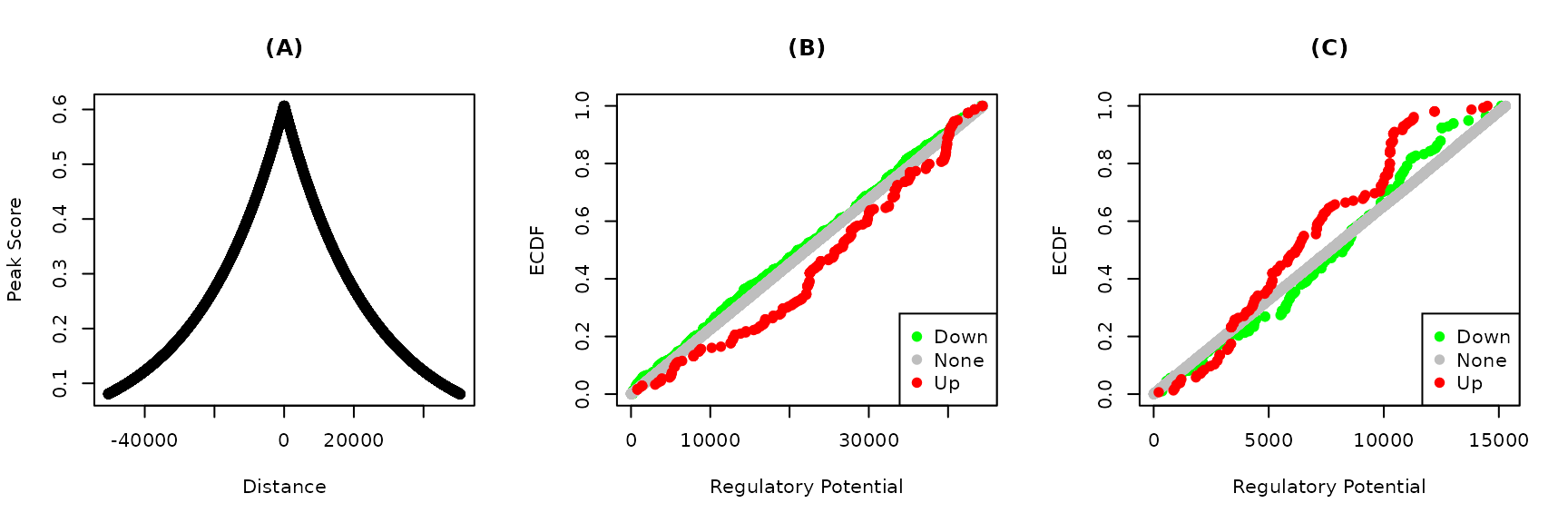
Figure 2. Predicted functions of YY1 and YY2 on their specific targets. Bindings peaks of the transcription factors in HeLa cells were determined using ChIP-Seq. Distances from the transcription start sites and the transformed distances of the (A) YY1 and YY2 peaks are shown. The regulatory potential of each gene was calculated using target. Genes were grouped into up, none or down regulated based on the fold-change. The emperical cumulative distribution functions (ECDF) of the groups of (C) YY1 and (D) YY2 targets are shown at each regulatory potential value.
The scores of the individual peaks are a decreasing function of the distance from the transcription start sites.
The closer the factor binding site from the start site the lower the score. The distribution of these scores is very similar for both factors (Figure 2A). The ECDF of the down-regulated targets of YY1 is higher than that of up- and none-regulated targets (Figure 2B). Therefore, the absence of YY1 on its targets result in aggregate in their down regulation.
The opposite is true for YY2 where more high ranking targets are up-regulated by the factor knockdown (Figure 2C).
# Table 2
# test individual factor functions
map2(dt, groups,
     ~test_predictions(.x$rank,
                       group = .y,
                       compare = c('Down', 'Up')))
#> $YY1
#>
#>  Two-sample Kolmogorov-Smirnov test
#>
#> data:  x and y
#> D = 0.78597, p-value < 2.2e-16
#> alternative hypothesis: two-sided
#>
#>
#> $YY2
#>
#>  Two-sample Kolmogorov-Smirnov test
#>
#> data:  x and y
#> D = 0.40354, p-value = 1.075e-12
#> alternative hypothesis: two-sided
To formally test these observations, we use the Kolmogorov-Smirnov (KS) test. The distribution of the two groups are compared for equality. If one lies one either side of the other then they must be drawn from different distributions.
Here, we compared the up- and down-regulated functions for both factors (Table 2).
In both cases, the distribution of the two groups were significantly different from one another.
Predicting the shared targets of the two factors
Similar to the previous analysis,
- Identify shared/common peaks using
subsetByOverlaps. - Pass two columns to
stats_colto use the fold-changes from both factors -
common_peaksandboth_regionsare the main inputs
# merge and name peaks
common_peaks <- GenomicRanges::reduce(subsetByOverlaps(peaks$YY1, peaks$YY2))
common_peaks$name <- paste0('common_peak_', 1:length(common_peaks))
# bind express tables into one
both_express <- bind_rows(express) %>%
  pivot_wider(names_from = tf,
              values_from = c(fc, pvalue))

# match symbols between genome and expression objects
ind <- match(genome$gene, both_express$gene)

# subset genome by genes with expression info
both_regions <- genome[genome$gene %in% both_express$gene]

# add expression info to gene info
mcols(both_regions) <- cbind(mcols(both_regions), both_express[ind,])
# get associated peaks with both factors
common_ap <- associated_peaks(peaks = common_peaks,
                              regions = both_regions,
                              regions_col = 'tx_id')
# get direct targets of both factors
common_dt <- direct_targets(peaks = common_peaks,
                            regions = both_regions,
                            regions_col = 'tx_id',
stats_col = c('fc_YY1', 'fc_YY2'))-
associated_peaksis the same as before. -
direct_targetsis the same but thestatand thestat_rankcarry the product of the two statistics provided in the previous step and the rank of that product.
The output can also be visualized the same way. The targets are divided into three groups based on the statistics product.
- When the two statistics agree in the sign, the product is positive. This means the knockdown of either transcription factor results in same direction change in the target gene expression. Therefore, the two factors would cooperate if they bind to the same site on that gene.
- The reverse is true for targets with opposite signed statistics. On these targets, the two factors would be expected to compete for inducing opposing changes in the expression.
# Figure 3
par(mfrow = c(1, 2))
# plot distiace by score for associated peaks
plot(common_ap$distance,
     common_ap$peak_score,
     xlab = 'Distance',
     ylab = 'Peak Score')
title('(A)')

# make labels, colors and gorups
labs <- c('Competitive', 'None', 'Cooperative')
cols <- c('green', 'gray', 'red')

# make three groups by quantiles
common_groups <- cut(common_dt$stat,
                     breaks = 3,
                     labels = labs)

# plot predicted function
plot_predictions(common_dt$score_rank,
                 group = common_groups,
                 colors = cols, labels = labs,
                 xlab = 'Regulatory Interaction', ylab = 'ECDF')
title('(B)')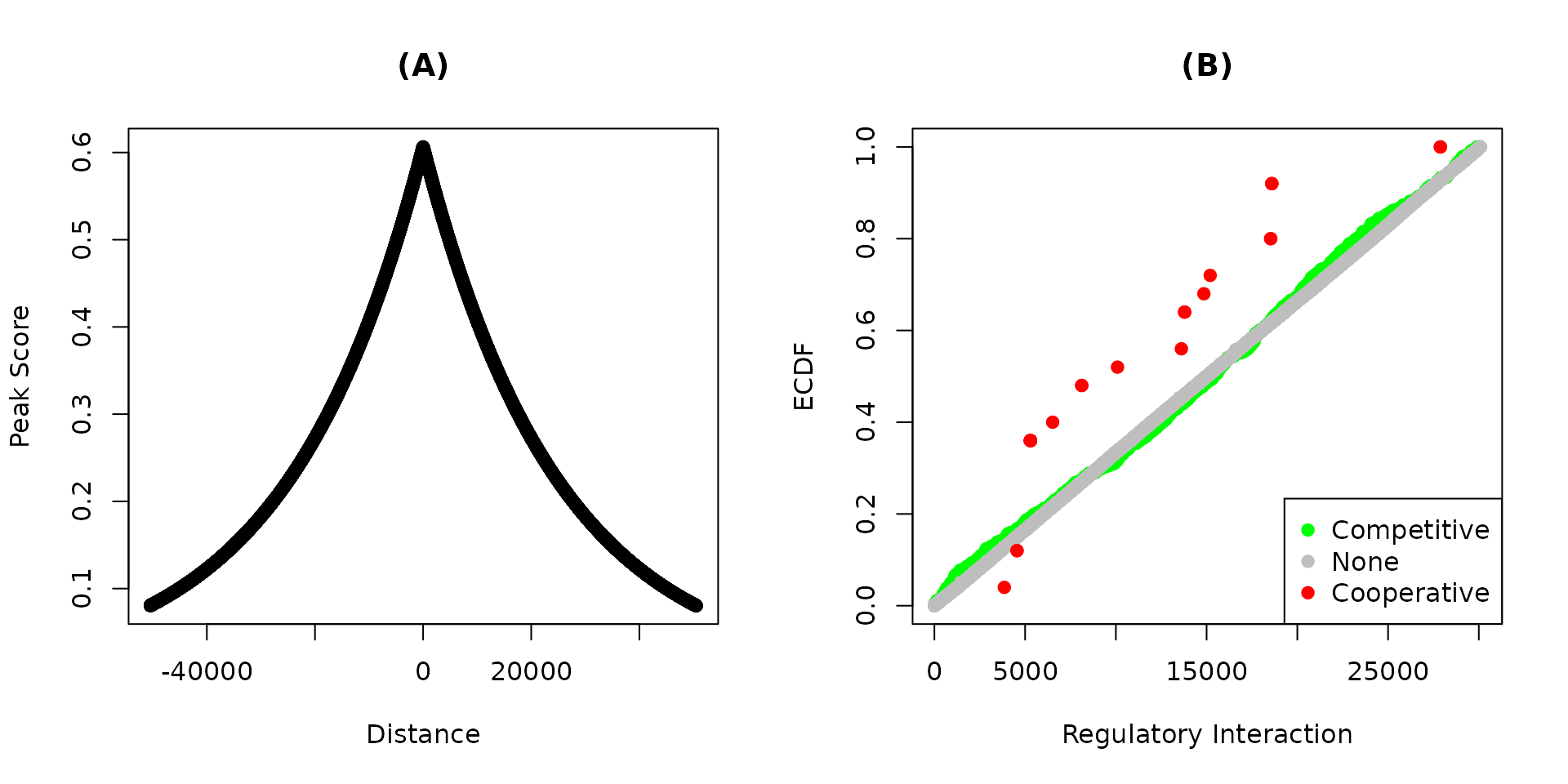
Figure 3. Predicted function of YY1 and YY2 on their shared targets. Shared bindings sites of YY1 and YY2 in HeLa cells were determined using the overlap of the individual factor ChIP-Seq peaks. (A) Distances from the transcription start sites and the transformed distances of the shared peaks are shown. The regulatory interaction of each gene was calculated using target. Genes were grouped into cooperatively, none or competitively regulated based on the the product of the fold-changes from YY1- and YY2-knockdown. (B) The emperical cumulative distribution functions (ECDF) of the groups of targets are shown at each regulatory potential value.
- The common peaks distances and scores take the same shape (Figure 3A).
- The two factors seem to cooperate on more of the common target than any of the two other possibilities (Figure 3B).
This observation can be tested using the KS test. The curve of the cooperative targets lies above that of none and competitively regulated targets (Table 3).
# Table 3
# test factors are cooperative
test_predictions(common_dt$score_rank,
                 group = common_groups,
                 compare = c('Cooperative', 'None'),
                 alternative = 'greater')
#>
#>  Two-sample Kolmogorov-Smirnov test
#>
#> data:  x and y
#> D^+ = 0.30253, p-value = 0.01034
#> alternative hypothesis: the CDF of x lies above that of y

# test factors are more cooperative than competitive
test_predictions(common_dt$score_rank,
                 group = common_groups,
                 compare = c('Cooperative', 'Competitive'),
                 alternative = 'greater')
#>
#>  Two-sample Kolmogorov-Smirnov test
#>
#> data:  x and y
#> D^+ = 0.29706, p-value = 0.01263
#> alternative hypothesis: the CDF of x lies above that of y
Summary
- I presented a workflow for predicting the direct targets of a transcription factor by integrating binding and expression data.
- The
targetpackage implements the BETA algorithm to rank targets based on the distance of the ChIP peaks of the transcription factor in the genes and the differential expression from the factor perturbation. - To predict the combined function of two factors, two sets of data are used to find the shared peaks and the product of their differential expression.
References
Chen, Li, Toshi Shioda, Kathryn R. Coser, Mary C. Lynch, Chuanwei Yang, and Emmett V. Schmidt. 2010. “Genome-wide analysis of YY2 versus YY1 target genes.” Nucleic Acids Research 38 (12): 4011–26. https://doi.org/10.1093/nar/gkq112.
Michaud, Joëlle, Viviane Praz, Nicole James Faresse, Courtney K Jnbaptiste, Shweta Tyagi, Frédéric Schütz, and Winship Herr. 2013. “HCFC1 is a common component of active human CpG-island promoters and coincides with ZNF143, THAP11, YY1, and GABP transcription factor occupancy.” Genome Research 23 (6): 907–16. https://doi.org/10.1101/gr.150078.112.
Wu, Xiao-Nan, Tao-Tao Shi, Yao-Hui He, Fei-Fei Wang, Rui Sang, Jian-Cheng Ding, Wen-Juan Zhang, et al. 2017. “Methylation of transcription factor YY2 regulates its transcriptional activity and cell proliferation.” Cell Discovery 3: 17035. https://doi.org/10.1038/celldisc.2017.35.